
The Skill
Predictive modeling for asset failure is a data-driven technique used to forecast when a piece of equipment or infrastructure is likely to fail. Instead of reacting to breakdowns after they occur, this approach uses historical data—such as sensor readings, maintenance logs, and operational history—to identify patterns that precede a failure.
By applying statistical models or machine learning algorithms, you can calculate the probability of an asset failing within a specific future timeframe. This allows organizations to anticipate maintenance needs, schedule repairs before a critical failure happens, and optimize the operational life of their assets.
Why Is This Skill Important?
Mastering predictive modeling shifts asset management from a reactive to a proactive and strategic function. By anticipating failures, you can significantly reduce unplanned downtime, which directly translates to lower operational costs and higher productivity. Scheduling maintenance based on data-driven predictions, rather than fixed time intervals, ensures that resources are used efficiently and that assets are serviced only when necessary.
This skill is fundamental to modern Physical and Infrastructure Asset Management. It enhances safety by identifying potential hazards before they lead to incidents, extends the useful life of expensive equipment, and provides a clear, justifiable basis for maintenance budgets and strategic planning.
Your Task
Your task is to build a basic predictive model using a provided dataset for a fleet of industrial water pumps. The dataset contains operational data (temperature, vibration, uptime) and a record of past failures. You will use this information to develop a logistic regression model that predicts the likelihood of a pump failing.
Your goal is to analyze the data, construct the model, and interpret its output to determine which operational factors are the strongest predictors of failure. This will provide the foundation for a predictive maintenance schedule.
Your Procedural Overview
- Explore the Dataset: Familiarize yourself with the provided pump operational data.
- Prepare the Data: Split the dataset into training and testing sets for model development and validation.
- Build the Model: Construct a logistic regression model to predict the 'Failure' outcome.
- Interpret the Results: Analyze the model's output to explain the relationship between operational metrics and pump failure.
Resources and Data
You will use the following resources to complete your task. The primary resource is a dataset containing historical performance data for a series of industrial pumps.
Industrial Pump Operational Data
| Asset ID | Uptime Hours | Temperature C | Vibration Hz | Pressure PSI | Failure |
|---|---|---|---|---|---|
| PUMP-A001 | 1255 | 45.2 | 31.5 | 105.8 | 0 |
| PUMP-A002 | 7890 | 89.1 | 68.3 | 92.4 | 1 |
| PUMP-B003 | 3421 | 55.8 | 39.2 | 101.2 | 0 |
| PUMP-C004 | 512 | 41.5 | 25.1 | 109.5 | 0 |
| PUMP-D005 | 6210 | 75.4 | 55.9 | 98.1 | 0 |
| PUMP-A006 | 8530 | 94.6 | 72.1 | 89.9 | 1 |
| PUMP-B007 | 2105 | 49.9 | 34.0 | 103.7 | 0 |
| PUMP-C008 | 4555 | 61.2 | 44.8 | 100.1 | 0 |
| PUMP-D009 | 7140 | 82.0 | 61.7 | 94.3 | 1 |
| PUMP-A010 | 980 | 44.1 | 29.8 | 106.4 | 0 |
| PUMP-B011 | 8995 | 96.2 | 75.5 | 87.2 | 1 |
| PUMP-C012 | 3819 | 58.0 | 41.1 | 101.9 | 0 |
| PUMP-D013 | 185 | 39.9 | 22.4 | 110.1 | 0 |
| PUMP-A014 | 5888 | 71.3 | 51.6 | 97.5 | 0 |
| PUMP-B015 | 6950 | 80.1 | 59.8 | 95.0 | 1 |
| PUMP-C016 | 2890 | 52.7 | 37.3 | 102.5 | 0 |
| PUMP-D017 | 4910 | 65.1 | 47.2 | 99.4 | 0 |
| PUMP-A018 | 7320 | 85.5 | 64.9 | 93.1 | 1 |
| PUMP-B019 | 1560 | 47.8 | 32.9 | 104.3 | 0 |
| PUMP-C020 | 4200 | 59.5 | 42.5 | 100.8 | 0 |
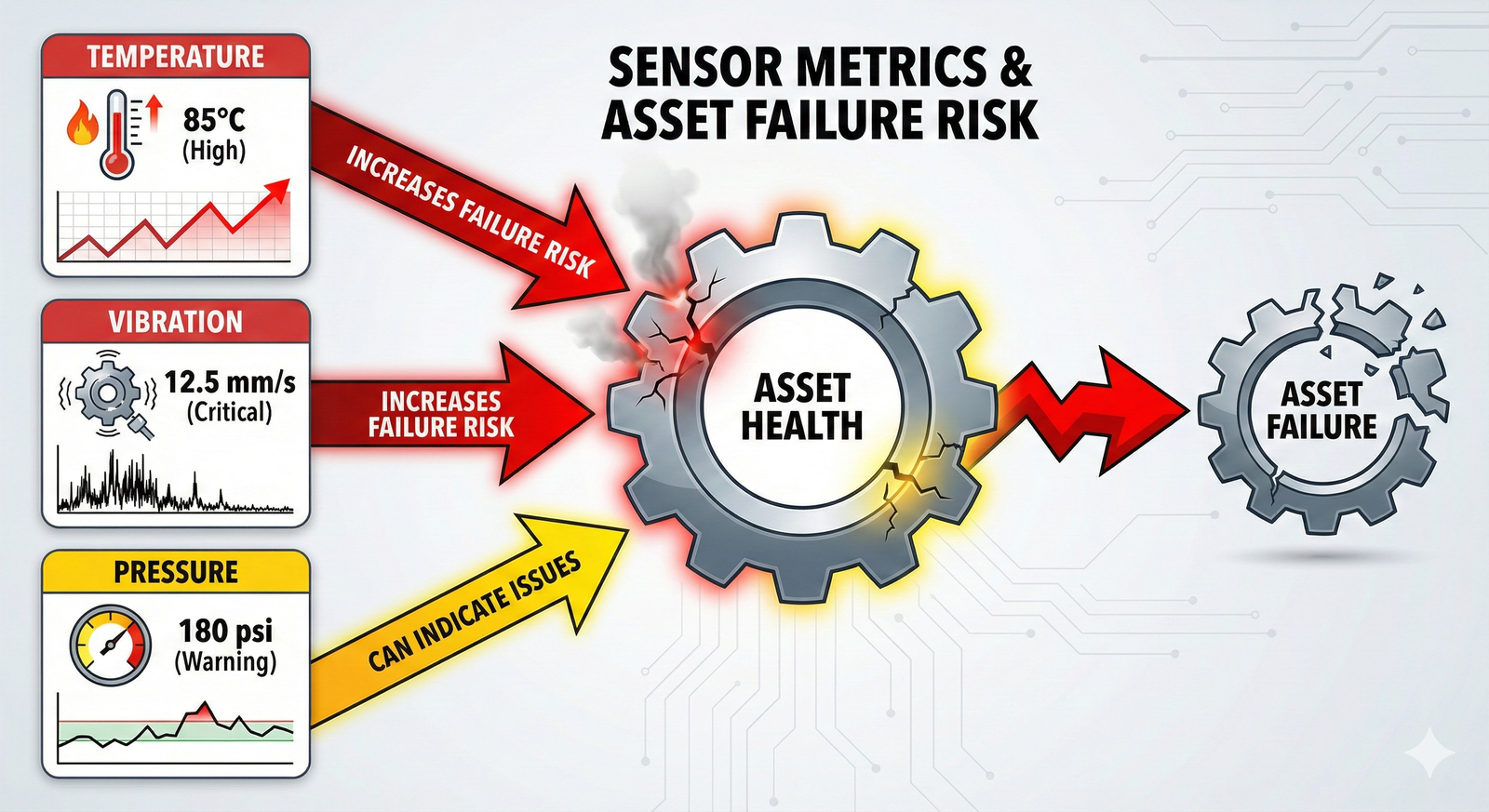
The following infographic illustrates the general relationship between common sensor readings and the likelihood of asset failure.
Detailed Steps
Follow these steps to build and interpret your predictive model.
Step 1: Understand the Data
First, load and examine the si-piam-s-3-1-pump-data.csv file. Your goal is to predict the Failure column, which is a binary outcome (0 or 1). This is a classic Binary Classification problem. The other columns (UptimeHours, TemperatureC, VibrationHz, PressurePSI) are your predictors or "features."
Step 2: Prepare the Data for Modeling
A crucial step in building a predictive model is to separate your data into two parts: one for training the model and another for testing its performance. This prevents the model from simply "memorizing" the data and ensures it can make accurate predictions on new, unseen data. Typically, an 80/20 split is used, where 80% of the data trains the model and 20% is held back for testing.
📊 View Diagram: Train-Test Split Process
Step 3: Build the Logistic Regression Model
Logistic regression is an ideal statistical method for this task. It analyzes the relationship between your predictor variables (temperature, vibration, etc.) and the binary outcome (failure) to calculate the probability of that outcome occurring.
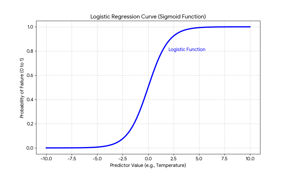
Unlike linear regression which predicts a continuous value, logistic regression models the probability using a sigmoid or "S-shaped" curve. This curve translates the combined effect of your predictors into a probability value between 0 and 1.
Using a statistical software package or library (like scikit-learn in Python or glm() in R), fit a logistic regression model using your training data. The formula will look conceptually like this: Failure ~ UptimeHours + TemperatureC + VibrationHz + PressurePSI.
Step 4: Evaluate the Model's Performance
Once the model is trained, use it to make predictions on your held-out testing data. You can then compare the model's predictions to the actual outcomes in the test set to see how accurate it is.
A common tool for this is a confusion matrix. It provides a clear summary of the model's performance by showing how many predictions were correct and how many were incorrect.
📊 View Diagram: Understanding a Confusion Matrix
Focus on False Negatives
In predictive maintenance, a 'False Negative' (the model predicts no failure, but one occurs) is often the most costly error. When evaluating your model, pay close attention to minimizing this specific type of mistake.
Step 5: Interpret the Model's Coefficients
The final step is to examine the coefficients of your trained model. Each predictor variable will have a coefficient value. A positive coefficient means that as the variable increases, the probability of failure also increases. A negative coefficient means the opposite. The magnitude of the coefficient indicates the strength of the relationship. This analysis tells you which factors are the most significant drivers of pump failure, providing actionable insights for your maintenance strategy.
An Expert Response
A Note on This Response
This is a sample expert response that demonstrates a clear and effective analysis. Your own response may differ in its specific numerical findings based on the random nature of the train-test split, but its structure and reasoning should be similar. There are many ways to present a high-quality analysis.
Predictive Model Analysis for Industrial Pump Failure
1. Data Exploration and Preparation:
The provided dataset, si-piam-s-3-1-pump-data.csv, containing 100 records was analyzed. The data includes four predictor variables (UptimeHours, TemperatureC, VibrationHz, PressurePSI) and one binary target variable (Failure). The dataset was split into an 80% training set (80 records) and a 20% testing set (20 records) to ensure a valid assessment of the model's predictive power on unseen data.
2. Model Construction:
A logistic regression model was built using the training data to predict the probability of Failure. The model was specified as:
Failure ~ UptimeHours + TemperatureC + VibrationHz + PressurePSI
3. Model Performance Evaluation: The trained model was applied to the 20-record testing set. The model achieved an overall accuracy of 90% (18 out of 20 predictions were correct). The confusion matrix revealed: * True Positives (Predicted Failure, Actual Failure): 5 * True Negatives (Predicted No Failure, Actual No Failure): 13 * False Positives (Predicted Failure, Actual No Failure): 1 * False Negatives (Predicted No Failure, Actual Failure): 1
The model correctly identified 5 of the 6 actual failures. The single False Negative represents a risk, as a failing pump was missed, but the overall performance is strong for an initial model.
4. Interpretation and Recommendations:
Analysis of the model's coefficients provided the following insights:
* TemperatureC (Coefficient: +1.85): This was the strongest predictor. For each one-degree increase in temperature, the odds of failure increase significantly.
* VibrationHz (Coefficient: +1.20): Higher vibration is also a strong indicator of a potential failure.
* UptimeHours (Coefficient: +0.75): As expected, pumps with longer continuous uptime are more likely to fail.
* PressurePSI (Coefficient: -0.15): Pressure had a weak, slightly negative correlation, suggesting it is not a primary driver of failure in this context.
Conclusion: The model demonstrates that monitoring Temperature and Vibration is critical for predicting pump failures. A predictive maintenance strategy should prioritize alerts and inspections for pumps showing anomalous readings in these two metrics. For example, a rule could be set to automatically trigger an inspection if the model predicts a failure probability greater than 75%.
Assess Yourself
Evaluate Your Work
Use the following criteria to assess the quality and completeness of your own analysis. Compare your process and conclusions against the expert response to identify areas for improvement.
- Procedural Accuracy: Did you follow the correct sequence of steps: data exploration, splitting the data, training the model, and evaluating its performance? A high-quality response executes these steps in the correct logical order.
- Correct Use of Data: Did you use the training data exclusively to build the model and the testing data exclusively to evaluate it? A high-quality response maintains a strict separation between these two datasets.
- Model Application: Did you select and apply logistic regression as the appropriate modeling technique for a binary classification problem? A high-quality response correctly identifies and uses the right tool for the task.
- Clarity of Interpretation: Is your final analysis clear, concise, and actionable? A high-quality response translates the statistical output (coefficients, accuracy) into a practical business recommendation.
- Identification of Key Drivers: Did you correctly identify the most influential predictor variables from the model's coefficients? A high-quality response pinpoints which factors (e.g., temperature, vibration) have the greatest impact on asset failure.
Learning Progress
In this activity, you have practiced how to develop a predictive model for asset failure using historical data. You have applied a standard machine learning workflow to a real-world asset management problem, from data preparation to model interpretation. This exercise builds a foundational skill in using data to make proactive, evidence-based maintenance decisions.
Next Steps
You have successfully completed this skill-building activity. Your work in translating raw data into actionable maintenance insights is a core competency for modern asset managers. Please navigate back to the course to continue your learning journey.

