
Introduction
Welcome. If you've ever had to make a multi-million dollar decision about an asset based on a spreadsheet that felt more like a house of cards, you're in the right place. We've all been there: trying to predict the future life of a critical pump, a bridge deck, or a power transformer with tools that assume the world operates in straight, predictable lines. But you know it doesn't. Equipment fails unexpectedly, repair costs fluctuate, and environmental conditions change.
This is where we move beyond basic forecasting and into the world of advanced analytical models. This isn't about abstract mathematics; it's about equipping you with a powerful framework to understand, quantify, and manage the inherent uncertainty in physical assets. In this reading, we will explore two of the most potent tools in the modern asset manager's arsenal: Monte Carlo Simulation and Optimization. These methods allow you to stop guessing and start modeling reality in all its complex, unpredictable glory. You'll learn how to answer not just "what is the likely cost?" but "what is the full range of possible costs, and what's the probability of a catastrophic budget overrun?" This is the skill that separates a good asset manager from a great one.
The Problem with Averages
Let's start with a foundational problem. Your team is responsible for a fleet of 500 identical water pumps. Historical data tells you that, on average, a pump costs $10,000 to replace and has a useful life of 15 years. For your annual budget, you might simply calculate the number of pumps reaching 15 years of age and multiply by $10,000. This is a deterministic approach—it assumes the inputs are fixed and known.
But what happens in the real world? Some pumps fail at 8 years, others last for 22. A supply chain disruption causes the replacement cost to spike by 30% for six months. A simple, average-based calculation can't account for this variability. It gives you a single, deceptively precise number that might be precisely wrong. The result? Unplanned failures, emergency procurements, and frantic calls to the finance department. To manage complex assets effectively, we must embrace and quantify uncertainty. This requires us to think in terms of probabilities and distributions, not just single-point averages.
Embracing Uncertainty: The Stochastic Approach
The world of asset management is inherently random, or stochastic. A stochastic process is one where the outcome is not fixed but follows a random probability distribution. The time it takes for a pipe to corrode to a critical point, the number of potholes that will form on a stretch of highway after a winter, the daily demand on a power substation—these are all stochastic variables.
Ignoring this randomness is a major source of risk. By acknowledging it, we can use advanced models to build more resilient and cost-effective asset management plans. This is where Monte Carlo simulation comes in.
From Deterministic to Probabilistic Thinking
The shift from deterministic to stochastic modeling is a fundamental step-up in analytical maturity. A deterministic model gives you one answer (e.g., 'The bridge will need resurfacing in 12.5 years'). A stochastic model gives you a range of answers and their probabilities (e.g., 'There is a 10% chance of needing resurfacing by year 8, a 50% chance by year 12, and a 90% chance by year 15'). This probabilistic output is far more valuable for risk management and long-term financial planning.
Monte Carlo Simulation: Gaming the System for Better Decisions
Imagine you could live the next 50 years of an asset's life a thousand times over. You could see all the different ways it could fail, all the different costs you might incur, and all the potential outcomes of your maintenance strategies. After running these thousand "lives," you could look at the aggregated results and have a crystal-clear picture of the most likely outcomes and the worst-case scenarios.
That is the essence of Monte Carlo Simulation. It's a method for turning uncertainty in your inputs into a probabilistic forecast of your outputs. The name, coined by physicists working on the atomic bomb in the 1940s, is a nod to the famous Monte Carlo casino, a center of games of chance.
How Does It Work?
Instead of using a single number for an uncertain variable (like the 15-year life of our pump), you define it as a probability distribution. For example, you might tell the model that the pump's life is "normally distributed with a mean of 15 years and a standard deviation of 3 years." You would do the same for other uncertain variables, like repair costs, which might follow a different type of distribution.
The simulation then runs a single "iteration" or "trial": 1. It plucks a random value for each uncertain variable from its defined probability distribution (e.g., it might pick a life of 17.2 years for the pump and a replacement cost of $9,850). 2. It calculates the outcome based on these specific values (e.g., the total cost for that single simulated scenario). 3. It records the result.
Now, repeat this process 10,000 times.
📊 View Diagram: The Monte Carlo Simulation Process
When you're done, you don't have a single answer. You have 10,000 answers. By plotting these 10,000 results on a histogram, you get a powerful output: a probability distribution of your potential outcomes. You can now answer questions like: * What is the mean expected cost for my pump replacement program next year? * What is the probability that my costs will exceed the budgeted amount by 20%? (This is your risk exposure). * What is the 90th percentile cost? (This is the number you might use to set a contingency budget, knowing there's only a 10% chance of exceeding it).
A Practical Example: Corrosion on a Pipeline
Let's make this tangible. You manage a 20-mile-long natural gas pipeline built in the 1980s. Your primary concern is external corrosion. A failure would be catastrophic. You need to decide on a budget for your inspection and rehabilitation program for the next decade.

Your uncertain variables are: * Corrosion Growth Rate: This isn't constant. It depends on soil moisture, pH, and temperature, which all vary. You can model this as a distribution based on historical data and soil samples. * Inspection Accuracy: Your "smart pig" inspection tool is good, but not perfect. There's a probability it will miss a defect (a false negative) or flag a harmless anomaly (a false positive). * Rehabilitation Cost: The cost to excavate and repair a section of pipe varies with location (is it under a road or in an open field?), labor rates, and material costs.
You can build a Monte Carlo model that simulates the growth of corrosion on thousands of virtual sections of your pipe over ten years. In each year of each simulation run, the model randomly decides if an inspection occurs, if it finds the (randomly grown) defect, and what the (randomly determined) cost of repair is.
After 10,000 runs, you can present a budget request not with a single number, but with a confidence curve. "I am 90% confident that our capital needs for this program over the next decade will not exceed $15.7 million. The expected value is $12.2 million, but there is a 5% chance of an extreme scenario costing over $20 million if we experience a series of rapid corrosion growths and coincident cost spikes." That is a powerful, defensible, and honest statement to make to a board of directors.
Table 1: Probabilistic Inputs for Pipeline Corrosion Model
| Parameter | Distribution Type | Value1 Mean | Value2 StdDev | Units |
|---|---|---|---|---|
| Corrosion Growth Rate | Lognormal | 0.1 | 0.05 | mm/year |
| Inspection Detection Probability | Uniform | 0.85 | 0.98 | Probability |
| Repair Cost per foot | Normal | 1500 | 250 | USD |
| Soil Resistivity | Lognormal | 5000 | 1500 | Ohm-cm |
| Coating Degradation Factor | Normal | 1.05 | 0.02 | Factor |
| Initial Defect Size | Normal | 2.5 | 0.5 | mm |
| Pipeline Operating Pressure | Normal | 1000 | 50 | psi |
| Failure Pressure | Lognormal | 1800 | 200 | psi |
From "What If" to "What's Best": An Introduction to Optimization
Monte Carlo simulation is fantastic for understanding the range of possible futures. But it doesn't, by itself, tell you what to do. It can show you the likely outcome of your current maintenance plan, but can it help you find a better one?
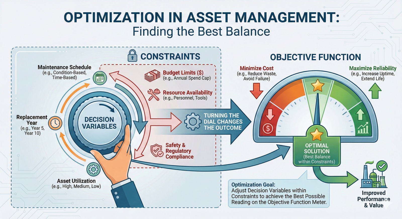
This is the domain of Optimization Models. An optimization model seeks to find the best possible decision by adjusting variables you control to achieve a specific objective, while respecting a set of constraints.
The classic structure of an optimization problem has three parts: 1. Objective Function: What are you trying to maximize or minimize? Examples: Minimize total lifecycle cost, maximize system reliability, minimize the number of service interruptions. 2. Decision Variables: What levers can you pull? Examples: Which pipes to replace this year, what level of maintenance to apply to each transformer, the inspection frequency for a bridge. 3. Constraints: What are your limitations? Examples: The annual capital budget cannot exceed $5 million, you only have 3 specialized repair crews available, a certain level of system performance must be maintained.
A Simple Optimization Example: Pavement Management
Imagine you are responsible for a road network. You have a budget of $1 million for this year. You have data on every road segment: its length, traffic volume, and current condition (Pavement Condition Index, or PCI). You also have a set of possible actions for each segment: * Do nothing * Crack sealing (low cost, small PCI improvement) * Mill and overlay (medium cost, medium PCI improvement) * Full reconstruction (high cost, PCI goes to 100)
Your objective is to maximize the average PCI of the entire network after your interventions. Your decision variables are which action to take on each and every road segment. Your constraint is that the total cost of all chosen actions must be less than or equal to $1 million.
You could try to solve this by hand or in a spreadsheet, but you'd quickly be overwhelmed. An optimization algorithm, like a Linear Program, can solve this problem in seconds. It will test thousands of combinations of projects to find the specific portfolio of work that gives you the biggest "bang for your buck"—the greatest overall improvement in network health for your limited budget.
The Power Couple: Combining Simulation and Optimization
The real magic happens when you combine these two techniques. Remember our pipeline corrosion problem? The Monte Carlo simulation gave us a probabilistic understanding of its degradation. Now, we can use that as an input to an optimization model.
The optimization model's objective could be to minimize the total 30-year lifecycle cost (inspections + repairs + risk of failure). The decision variables would be the timing of inspections and the criteria for when to trigger a repair (e.g., "repair any defect with a predicted depth greater than 50% of the wall thickness"). The model would run thousands of combinations of inspection schedules and repair criteria, using the Monte Carlo engine under the hood to evaluate the long-term cost and risk of each strategy.
The final output isn't just a budget, but an optimized strategy: "The lowest total lifecycle cost is achieved with a 7-year inspection interval and a repair threshold of 40% wall loss. This strategy results in an expected 30-year cost of $45 million, with a 95% confidence of being below $60 million." You have now used advanced analytics to create a data-driven, risk-informed, and economically optimized asset management plan. This is the pinnacle of strategic asset management.
A Word of Caution: Garbage In, Garbage Out (GIGO)
These models are incredibly powerful, but they are not magic. The quality of your output is entirely dependent on the quality of your input. If your historical data is poor, or if you make unrealistic assumptions about your probability distributions, your model will produce flawed results, no matter how sophisticated it is. A significant part of applying these techniques successfully is the hard work of collecting good data, understanding the underlying physical processes, and validating your model's assumptions.
Closing
We've covered a lot of ground, moving from the simple world of deterministic averages to the more realistic and powerful realm of stochastic analysis. You've seen how Monte Carlo simulation allows you to quantify uncertainty and understand the full spectrum of potential outcomes, transforming your risk conversations from vague concerns into specific probabilities. We then saw how optimization models provide a structured way to find the best course of action within your real-world constraints.
The true power, as we've discussed, lies in combining these approaches to develop strategies that are not only economically efficient but also resilient in the face of an uncertain future. Applying these analytical models is a core competency for the modern asset management professional. It's the foundation for moving your organization from a reactive, fire-fighting culture to a proactive, strategic one. The journey requires a commitment to data and a new way of thinking, but the payoff—in improved safety, reliability, and financial performance—is immense.
Learning Outcomes
In this reading, you have explored the foundational concepts required to apply advanced analytical models to support your asset management decisions. You now have a practical understanding of: * Stochastic Modeling: You can now articulate why incorporating randomness and probability is essential for realistically modeling physical assets. * Monte Carlo Simulation: You can explain how this technique uses repeated random sampling to turn uncertain inputs into a probabilistic forecast, allowing for sophisticated risk and cost analysis. * Optimization Models: You can describe how to frame a decision problem with an objective function, decision variables, and constraints to find the best possible solution.
By grasping these methods, you are better prepared to develop and defend robust, data-driven asset management strategies.
Assess Yourself
❓ Knowledge Check
Test your understanding of the key concepts from this section.
Next Steps
You have successfully completed this introduction to advanced analytical models. These concepts are foundational for making sophisticated, data-informed decisions in asset management. Take a moment to reflect on how you might apply this thinking to a familiar asset in your own experience. When you are ready, please navigate back to the course page to continue your learning journey.
